
Quantitative History, Spatial Heterogeneity, and the Problem of Generalization
By Adam Slez
One of the things that I love about historical political economy is the variety of methods that are brought to bear on historical materials. This includes quantitative methods such as regression. The emergence of quantitative history as a recognizable practice was due in no small part to the new political history movement of the 1960s, which saw historians consciously importing techniques from the social sciences into their home discipline. Perhaps the best-known example of this is Lee Benson, whose famed article “Research Problems in American Historiography” grew out of work funded by sociologist Paul Lazarsfeld and the Bureau of Applied Social Research at Columbia University (see Bogue 1968). Lazarsfeld’s contributions to the development of quantitative sociology in the postwar period are well-known. To the extent that the new political history movement was an outgrowth of the influence of Lazarsfeld and the Columbia School, the push to institutionalize quantitative history can be understood as an outgrowth of the quantification of the social sciences more generally.
The arrival of quantitative history was not without its critics. For many traditional historians, the problem was with quantification itself (see Ruggles 2021 for a review). Among historically-minded social scientists, the problem was less with quantification per se than it was with how the resulting analysis was usually done. Members of the latter group took particular issue with the use of global regression models that assigned a single parameter to each predictor. Their contention was that the conventional global model is fundamentally ahistorical insofar it ignores the types of contextual effects that have traditionally defined historical analysis. From this perspective, the way to make regression more historical is to allow for parameter heterogeneity. This line of argument is well-developed in the literature on time-series data, where time-varying parameter models have become commonplace, thanks to the pioneering efforts of scholars such as Isaac and Griffin (1989), among others. In a forthcoming article in Social Science History, I show how existing work on the connection between parameter heterogeneity and historical explanation can be extended to the case of space using a technique known as random effects eigenvector spatial filtering, which can be understood as low-rank approximation of a Bayesian spatially-varying coefficient model. To illustrate the utility of this approach, I revisit a critical case in the field of quantitative history—the rise of the electoral Populism in the American West.
I had been thinking and writing about spatial heterogeneity for years before this paper was accepted, but constantly struggled to explain why it was so important to allow parameters to vary from one place to the next. With the help of two anonymous reviewers, I was finally able to articulate the central problem with an uncritical reliance on the conventional global model, which is that we risk mistaking the simple and mathematically particular for the historically general. To get a sense of what is at stake, consider the figure below, which depicts the estimated marginal effect of wheat dependence on the average county-level vote share received by Populist gubernatorial candidates across five western states between 1890 and 1896 based on a global model, as compared to a series of state-specific models. Each model includes controls for mortgage prevalence and ethnic composition. The global model also includes controls for state membership, meaning that the intercept is allowed to vary by state, while all the other parameters are treated as fixed, producing a single estimate for each.
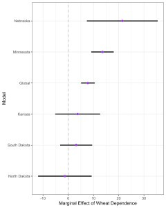
Looking at this figure, we see that the global estimate falls in the middle of the set of state-specific estimates, as we would expect. While this estimate is undeniably typical in a mathematical sense, it is unclear whether we can reasonably treat this as a general statement about the relationship between wheat dependence and electoral Populism across the states in question. This question gets a bit complicated once we begin to account for uncertainty in the estimates, but from a purely descriptive perspective, it is hard to imagine treating the global estimate as an accurate summary of what is happening in each of the other states. This especially true when considering the results at the extremes (i.e., North Dakota and Nebraska). To be clear, we don’t expect the set of state-specific effects to be exactly equal. A joint F-test confirms that the variation in state-specific parameter estimates is greater than what we would expect by chance alone, providing support for the claim that the marginal effect of wheat dependence was characterized by spatial instability. The key point is that as the distribution of effects becomes increasingly heterogenous, the typical estimate produced by the global model speaks to a smaller share of cases. In this context, it is impossible to produce a conclusion that is both simple and general (see Griffin 1992). This is not a problem with the analysis—it is a reflection of the conditions in the world that we are studying.
The analysis above focuses on discrete heterogeneity in the form of state-specific effects. All this requires is estimating separate models for each state or including a full range of interactions, depending on what you are willing to assume about the variance of the errors. In the paper, I use random effects eigenvector spatial filtering to allow for continuous heterogeneity in the form of county-specific effects. The ability to get a separate set of parameter estimates for each county may seem like magic, but the basic intuition follows naturally from a more conventional varying-intercept, varying-slope model. The difference is that rather than treating the set of local parameter estimates as independent draws from a common distribution, we use information on the spatial arrangement of observations to allow each case to borrow strength from its neighbors. Without getting into the gory details, what sets the random effects eigenvector spatial filtering approach apart from a traditional Bayesian spatially-varying coefficient model is that the random effects eigenvector spatial filtering model introduces the spatial information in question as a set of observed covariates, substantially reducing the time required to estimate the model.
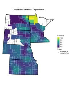
The map below depicts the set of local parameter estimates associated with wheat dependence. These estimates come from a model in which the effects of state membership are treated a constant, while the other parameters making up the linear predictor are allowed to vary across counties. As you can see, the estimated relationship between wheat dependence and electoral Populism is considerably weaker in most locales than what we would expect from the global model. To put things in perspective, while the global model suggests that a two-standard deviation change in the percentage of improved land dedicated to wheat production was associated with a nearly eight percentage point increase in the size of the expected Populist vote share, this figure drops to just two percentage points when looking at the average local effect. Remarkably, the magnitude of the local marginal effect remains fairly stable over large swaths of territory. The chief exception is in the handful of counties lying in the northwest corner of Minnesota—the one place where the relationship suggested by the global model seems to hold.
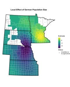
As I discuss in the paper, the marked difference in the magnitude of the global parameter estimate and the average local estimate is driven by the inclusion of a spatially-varying intercept, which serves as a correction for spatial dependence (Tiefelsdorf and Griffith 2007). It is worth noting that this divergence is unique to wheat dependence. This is not to say that the other sets of parameter estimates are unaffected by the introduction of spatially-varying parameters, as evidenced by the figure below, which depicts the set of local parameter estimates associated with the size of the German population.[1] More specifically, while the average local effect of the size of the German population is consistent with the parameter estimate produced by the global model (not shown), the distribution of local effects is characterized by large-scale variation, becoming more negative as we move away from southern Minnesota and Minneapolis-St. Paul and less negative as we move away from the area around Yankton, South Dakota, which is located in southeastern South Dakota, just north of the Nebraska border. In this setting, it is impossible to see how any one parameter estimate could reasonably serve as the basis for a general claim about the relationship between the size of the German population and the success of Populist candidates.
There is lots more in the paper in terms of both methodical and substantive discussion. In future posts, I would like to circle back to the differences between the various methods for modeling spatially-varying relationships, as well as to questions regarding the threat of overfitting, which can be addressed through the use of model averaging. For now, I want to reiterate that paying attention to spatial heterogeneity is about far more than striving for detail. The problems with the global model highlighted above were not a product of small differences. They were the result of large-scale variation in the underlying data generating process—variation that is typically ignored when using a conventional global model. This poses a significant challenge in the context of social science where heterogeneity is the rule, rather than the exception (see Gelman 2015). In this respect, the outmoded desire to produce simple conclusions runs head-to-head with a world that is anything but. Spatially-varying coefficient models are just one way forward, with the important caveat that the ability to capture spatial heterogeneity is not so much an end in its own right as it is a first step in making sense of what needs to be explained.
[1] This variable is reverse coded in the paper for the sake of visualization